Identifying duplicate entries in Google Sheets is essential for maintaining clean and accurate data. Here are straightforward methods suitable for beginners.
Using Conditional Formatting (Visual Highlight)
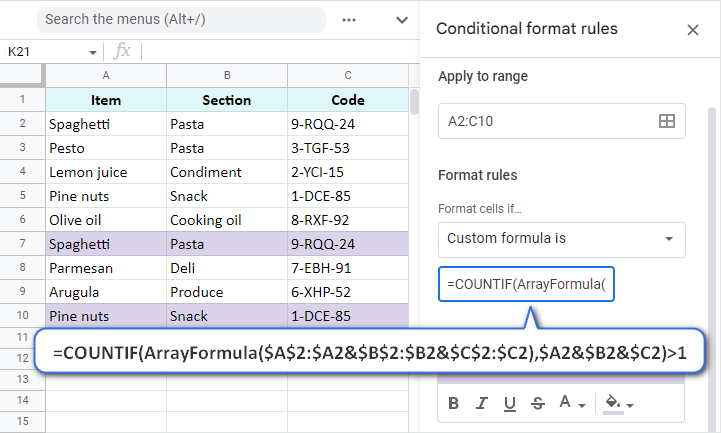
This method visually marks duplicate cells or rows for easy identification:
- Select the range of cells you want to check (e.g., A2:A100).
- Navigate to Format > Conditional formatting.
- Under the "Format rules" section, select "Custom formula is".
- Enter the formula:
=COUNTIF(A:A, A2)>1(Ensure the column reference matches your data). - Choose a highlighting style (e.g., red fill).
- Click "Done". Cells appearing more than once will be highlighted.
Using the UNIQUE Function (Simple List Extraction)
Quickly generate a list containing only unique values from your original data:
- Click on a blank cell where you want the unique list to start.
- Enter the formula:
=UNIQUE(A2:A100)(Adjust the range A2:A100 to match your data). - Press Enter. The formula outputs a spill range listing each unique entry only once.
- Compare the number of entries in the unique list versus the original to detect duplicates.
Using COUNTIF (Flag with Helper Column)
Add a column indicating how many times each entry appears:
- Insert a new column next to your data (e.g., Column B if data is in Column A).
- In the first cell of the new column (e.g., B2), enter:
=COUNTIF(A$2:A$100, A2). - Double-click the small blue square in the bottom-right corner of cell B2 to fill down the formula.
- Values in the helper column show the count. Any number greater than 1 indicates a duplicate.
- You can then sort or filter Column B to view duplicates easily.
Key Tips:
- Ensure consistent casing and formatting in your data; "apple" and "Apple" are treated as different.
- Always verify full rows: Duplicates might involve multiple columns. Use
=COUNTIFS(A$2:A$100, A2, B$2:B$100, B2)to check combinations. - Regularly audit your data using one of these methods to prevent error accumulation.